搜索到
486
篇与
的结果
-
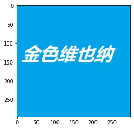
 七、图像金字塔与轮廓检测 七、图像金字塔与轮廓检测1. 图像轮廓(1)概念cv2.findContours(img, mode, method)mode(轮廓检测模式):RETR_EXTERNAL:只检测最外面的轮廓RETR_LIST:检测所有的轮廓,并将其保存到链表中RETR_CCOMP:检索所有的轮廓,并将他们组织为两层,第一层为各部分的外部边界,第二层为空洞的边界RETR_TREE:检索所有的轮廓,并重构嵌套轮廓的整个层次method(轮廓逼近的方法):CHAIN_APPROX_NONE:以 Freeman 链码的方式输出轮廓,所有其他方法输出多边形(顶点的序列)CHAIN_APPROX_SIMPLE:压缩水平的、垂直的和斜的部分,即函数只保留他们的终点部分import cv2 # OpenCV 读取的格式是 BGR import matplotlib.pyplot as plt import numpy as np %matplotlib inline img = cv2.imread('ysg.png') gray = cv2.cvtColor(img, cv2.COLOR_BGR2GRAY) # 使用二值图像提高准确率 ret, thresh = cv2.threshold(gray, 127, 255, cv2.THRESH_BINARY) plt.imshow(thresh, cmap='gray') plt.show()binary, contours, hierarchy = cv2.findContours(thresh, cv2.RETR_TREE, cv2.CHAIN_APPROX_NONE)(2)轮廓绘制img_cp = img.copy() # 参数:需绘制的图像,轮廓(-1为绘制所有轮廓),颜色模式,线条厚度 res = cv2.drawContours(img_cp, contours, -1, (0, 0, 255), 1) plt.imshow(cv2.cvtColor(res, cv2.COLOR_BGR2RGB)) plt.show()(3)轮廓特征cnt = contours[0] # 面积 cv2.contourArea(cnt) 136.0# 周长,True表示闭合 cv2.arcLength(cnt, True) 49.656854152679442. 模板匹配(1)概念模板匹配类似于卷积原理,模板在原图像上从原点开始滑动,计算模板与(图像被覆盖的地方)的差别程度(OpenCV中共6种计算方法),然后将每一次计算结果放入一个矩阵,作为结果输出。6种计算方法:TM_SQDIFF:计算平方不同,计算结果值越小,越相关TM_CCORR:计算相关性,计算结果值越大,越相关TM_CCOEFF:计算相关系数,计算结果值越大,越相关TM_SQDIFF_NORMED:计算归一化平方不同,计算结果值越接近0,越相关TM_CCORR_NORMED:计算归一化相关性,计算结果值越接近1,越相关TM_CCOEFF_NORMED:计算归一化相关系数,计算结果值越接近1,越相关如:原图像大小为 A x B,模板大小为 a x b,则输出结果矩阵是(A - a + 1) x (B - b + 1)img = cv2.imread('ysg.png', 0) template = cv2.imread('ysg_template.png', 0) h, w = template.shape[:2]img.shape (310, 341)template.shape (161, 144)res = cv2.matchTemplate(img, template, cv2.TM_SQDIFF) res.shape (150, 198)min_val, max_val, min_loc, max_loc = cv2.minMaxLoc(res) # 最小值 min_val 0.0 # 最大值 max_val 217423616.0 # 最小值位置 min_loc (67, 10) # 最大值位置 max_loc (189, 97)(2)示例methods = ['cv2.TM_SQDIFF', 'cv2.TM_CCORR', 'cv2.TM_CCOEFF', 'cv2.TM_SQDIFF_NORMED', 'cv2.TM_CCORR_NORMED', 'cv2.TM_CCOEFF_NORMED'] for item in methods: img_copy = img.copy() # 匹配方法的真值 method = eval(item) print(method) res = cv2.matchTemplate(img, template, method) min_val, max_val, min_loc, max_loc = cv2.minMaxLoc(res) # 如果平方差匹配TM_SQDIFF,或归一化平方差匹配TM_SQDIFF_NORMED,取最小值 if method in [cv2.TM_SQDIFF, cv2.TM_SQDIFF_NORMED]: top_left = min_loc else: top_left = max_loc bottom_right = (top_left[0] + w, top_left[1] + h) cv2.rectangle(img_copy, top_left, bottom_right, 255, 2) plt.subplot(121), plt.imshow(res, cmap='gray') plt.xticks([]), plt.yticks([]) plt.subplot(122), plt.imshow(img_copy, cmap='gray') plt.xticks([]), plt.yticks([]) plt.suptitle(item) plt.show()# 匹配多个对象 match = cv2.imread('ysg_match.png') match_gray = cv2.cvtColor(match, cv2.COLOR_BGR2GRAY) template = cv2.imread('ysg_template.png', 0) h, w = template.shape[:2] res = cv2.matchTemplate(match_gray, template, cv2.TM_CCOEFF_NORMED) threshold = 0.8 loc = np.where(res >= threshold) # 筛选匹配程度大于等于80%的 for pt in zip(*loc[::-1]): bottom_right = (pt[0] + w, pt[1] + h) cv2.rectangle(match, pt, bottom_right, (0, 0, 255), 1) plt.imshow(cv2.cvtColor(match, cv2.COLOR_BGR2RGB)) plt.show()3. 图像金字塔高斯金字塔向下采样(缩小)# 向下采样 img_down = cv2.pyrDown(img) plt.imshow(cv2.cvtColor(img_down, cv2.COLOR_BGR2RGB)) plt.show()img.shape (310, 341, 3) img_down.shape (155, 171, 3)向上采样(放大)# 向上采样 img = cv2.imread('ysg.png') img_up = cv2.pyrUp(img) plt.imshow(cv2.cvtColor(img_up, cv2.COLOR_BGR2RGB)) plt.show()img.shape (310, 341, 3) img_up.shape (620, 682, 3)拉普拉斯金字塔img = cv2.imread('ysg.png') down = cv2.pyrDown(img) down_up = cv2.pyrUp(down) if img.shape != down_up.shape: img = cv2.resize(img, (down_up.shape[1], down_up.shape[0])) res = img - down_up plt.imshow(cv2.cvtColor(res, cv2.COLOR_BGR2RGB)) plt.show()4. 轮廓近似outline = cv2.imread('outline.png') gray = cv2.cvtColor(outline, cv2.COLOR_BGR2GRAY) ret, thresh = cv2.threshold(gray, 127, 255, cv2.THRESH_BINARY) binary, contours, hierarchy = cv2.findContours(thresh, cv2.RETR_TREE, cv2.CHAIN_APPROX_NONE) cnt = contours[0] outline_cp = outline.copy() res = cv2.drawContours(outline_cp, [cnt], -1, (0, 0, 255), 2) plt.imshow(cv2.cvtColor(res, cv2.COLOR_BGR2RGB)) plt.show()# 值越小,越接近原始轮廓 epsilon = 0.1 * cv2.arcLength(cnt, True) approx = cv2.approxPolyDP(cnt, epsilon, True) outline_cp1 = outline.copy() res = cv2.drawContours(outline_cp1, [approx], -1, (0, 0, 255), 2) plt.imshow(cv2.cvtColor(res, cv2.COLOR_BGR2RGB)) plt.show()5. 边界矩形outline = cv2.imread('outline.png') gray = cv2.cvtColor(outline, cv2.COLOR_BGR2GRAY) ret, thresh = cv2.threshold(gray, 127, 255, cv2.THRESH_BINARY) binary, contours, hierarchy = cv2.findContours(thresh, cv2.RETR_TREE, cv2.CHAIN_APPROX_NONE) cnt = contours[0] x, y, w, h = cv2.boundingRect(cnt) res = cv2.rectangle(outline, (x, y), (x + w, y + h), (0, 0, 255), 2) plt.imshow(cv2.cvtColor(res, cv2.COLOR_BGR2RGB)) plt.show()# 轮廓面积与边界矩形比 area = cv2.contourArea(cnt) x, y, w, h = cv2.boundingRect(cnt) rect_area = w * h extent = float(area) / rect_area print(extent) 0.50601736972704716. 外接圆(x, y), radius = cv2.minEnclosingCircle(cnt) center = (int(x), int(y)) radius = int(radius) res = cv2.circle(res, center, radius, (0, 0, 255), 2) plt.imshow(cv2.cvtColor(res, cv2.COLOR_BGR2RGB)) plt.show()
 -
六、Canny 边缘检测 1. 流程(1) 使用高斯滤波器,以平滑图像,滤除噪声(2) 计算图像中每个像素点的梯度强度和方向(3) 应用非极大值(Nono-Maximum Suppression)抑制,以消除边缘检测带来的杂散响应(4) 应用双阈值(Double-Threshold)检测来确定真实的和潜在的边缘(5) 通过抑制孤立的弱边缘最终完成边缘检测2. 高斯滤波器3. 梯度和方向4. 非极大值抑制线性插值法设g1的梯度幅值M(g1),g2的梯度幅值M(g2),则dtmp1可以得到:M(dtmp1) = w x M(g2) + (1-w) x M(g1)其中w = distance(dtmp1, g2)/distance(g1, g2)distance(g1, g2) 表示两点之间的距离简化为了简化计算,由于一个像素周围有八个像素,可以将一个像素的梯度方向离散为八个方向,如此一来计算前后即可,简化插值法5. 双阈值检测梯度值 > maxVal:则该点处理为边界minVal < 梯度值 < maxVal:与现有的点(A点、C点)有关联(能连线),则保留,否则舍弃(B点)梯度值 < minVal:舍弃6. 演示import cv2 # OpenCV 读取的格式是 BGR import matplotlib.pyplot as plt import numpy as np %matplotlib inline img = cv2.imread('ysg.png', cv2.IMREAD_GRAYSCALE) plt.imshow(img, cmap='gray') plt.show() # 参数说明:源图,最小值,最大值 c1 = cv2.Canny(img, 60, 150) plt.imshow(c1, cmap='gray') plt.show() c2 = cv2.Canny(img, 50, 95) plt.imshow(c2, cmap='gray') plt.show() # 阈值范围越小细节越多
-
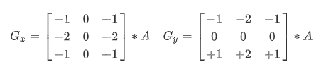
五、图像梯度计算 1. Sobel算子共p1,p2,p3,p4,p5,p6,p7,p8,p9 九个像素值Gx = p3 - p1 + 2 x p6 - 2 x p4 + p9 - p7Gy = p9 + 2 x p8 + p7 - p3 - 2 x p2 - p1import cv2 # OpenCV 读取的格式是 BGR import matplotlib.pyplot as plt import numpy as np %matplotlib inlineimg = cv2.imread('yuan.jpg', cv2.IMREAD_GRAYSCALE) # cv2.imshow('img', img) # cv2.waitKey(0) # cv2.destroyAllWindows() plt.imshow(img, cmap='gray') plt.show()dst = cv2.Sobel(src, ddepth, dx, dy, ksize)src:源图像ddepth:图像的深度dx:水平方向dy:垂直方向ksize:Sobel算子的大小sobel_x = cv2.Sobel(img, cv2.CV_64F, 1, 0, ksize=3) # cv2.imshow('sobel_x', sobel_x) # cv2.waitKey(0) # cv2.destroyAllWindows() # 白 --> 黑 是正数,黑 --> 白 是负数,负数会被截断为0,需要进行绝对值转换 sobel_abs_x = cv2.convertScaleAbs(sobel_x) plt.imshow(sobel_abs_x, cmap='gray') plt.show()sobel_y = cv2.Sobel(img, cv2.CV_64F, 0, 1, ksize=3) # cv2.imshow('sobel_y', sobel_y) # cv2.waitKey(0) # cv2.destroyAllWindows() # 白 --> 黑 是正数,黑 --> 白 是负数,负数会被截断为0,需要进行绝对值转换 sobel_abs_y = cv2.convertScaleAbs(sobel_y) plt.imshow(sobel_abs_y, cmap='gray') plt.show()# 分别计算x和y,再求和 sobel_x_y = cv2.addWeighted(sobel_display_x, 0.5, sobel_display_y, 0.5, 0) plt.imshow(sobel_x_y, cmap='gray') plt.show()例:分别计算和整体计算的效果进行对比ble = cv2.imread('ble.jpg', cv2.IMREAD_GRAYSCALE) # cv2.imshow('ble', ble) # cv2.waitKey(0) # cv2.destroyAllWindows() plt.imshow(ble, cmap='gray') plt.show()# 分别计算 (建议的操作方式) ble_sobel_x = cv2.Sobel(ble, cv2.CV_64F, 1, 0, ksize=3) ble_sobel_y = cv2.Sobel(ble, cv2.CV_64F, 0, 1, ksize=3) ble_sobel_abs_x = cv2.convertScaleAbs(ble_sobel_x) ble_sobel_abs_y = cv2.convertScaleAbs(ble_sobel_y) ble_sobel_x_y = cv2.addWeighted(ble_sobel_abs_x, 0.5, ble_sobel_abs_y, 0.5, 0) plt.imshow(ble_sobel_x_y, cmap='gray') plt.show()# 整体计算 ble_sobel_xy = cv2.Sobel(ble, cv2.CV_64F, 1, 1, ksize=3) ble_sobel_abs_xy = cv2.convertScaleAbs(ble_sobel_xy) plt.imshow(ble_sobel_abs_xy, cmap='gray') plt.show()2. Scharr算子共 p1,p2,p3,p4,p5,p6,p7,p8,p9 九个像素值Gx = 3 x p3 - 3 x p1 + 10 x p6 - 10 x p4 + 3 x p9 - 3 x p7Gy = -3 x p1 - 10 x p2 - 3 x p3 - 3 x p7 - 10 x p8 - 3 x p9ble_scharr_x = cv2.Scharr(ble, cv2.CV_64F, 1, 0) ble_scharr_y = cv2.Scharr(ble, cv2.CV_64F, 0, 1) ble_scharr_abs_x = cv2.convertScaleAbs(ble_scharr_x) ble_scharr_abs_y = cv2.convertScaleAbs(ble_scharr_y) ble_scharr_x_y = cv2.addWeighted(ble_scharr_abs_x, 0.5, ble_scharr_abs_y, 0.5, 0) plt.imshow(ble_scharr_x_y, cmap='gray') plt.show()3. Laplacian算子共 p1,p2,p3,p4,p5,p6,p7,p8,p9 九个像素值G = p2 + p6 - 4 x p5 + p3 + p8ble_laplacian = cv2.Laplacian(ble, cv2.CV_64F) ble_laplacian_abs = cv2.convertScaleAbs(ble_laplacian) plt.imshow(ble_laplacian_abs, cmap='gray') plt.show()
-
四、图像形态学操作 1. 腐蚀操作import cv2 # OpenCV 读取的格式是 BGR import matplotlib.pyplot as plt import numpy as np %matplotlib inlineimg = cv2.imread('jswyn.jpg') # cv2.imshow('img', img) # cv2.waitKey(0) # cv2.destroyAllWindows() plt.imshow(cv2.cvtColor(img, cv2.COLOR_BGR2RGB))<matplotlib.image.AxesImage at 0x2917d142438>kernel = np.ones((3, 3), np.uint8) erosion = cv2.erode(img, kernel, iterations=2) # cv2.imshow('erosion', erosion) # cv2.waitKey(0) # cv2.destroyAllWindows() plt.imshow(cv2.cvtColor(erosion, cv2.COLOR_BGR2RGB))<matplotlib.image.AxesImage at 0x2917e451dd8>yuan = cv2.imread('yuan.jpg') # cv2.imshow('yuan', yuan) # cv2.waitKey(0) # cv2.destroyAllWindows() plt.imshow(cv2.cvtColor(yuan, cv2.COLOR_BGR2RGB))<matplotlib.image.AxesImage at 0x2917df154a8>kernel = np.ones((3, 3), np.uint8) erosion_1 = cv2.erode(yuan, kernel, iterations=1) plt.imshow(cv2.cvtColor(erosion_1, cv2.COLOR_BGR2RGB))<matplotlib.image.AxesImage at 0x2917e749828>erosion_2 = cv2.erode(yuan, kernel, iterations=2) plt.imshow(cv2.cvtColor(erosion_2, cv2.COLOR_BGR2RGB))<matplotlib.image.AxesImage at 0x2917e791048>erosion_3 = cv2.erode(yuan, kernel, iterations=3) plt.imshow(cv2.cvtColor(erosion_3, cv2.COLOR_BGR2RGB))<matplotlib.image.AxesImage at 0x2917e7caa58>2. 膨胀操作img = cv2.imread('jswyn.jpg') # cv2.imshow('img', img) # cv2.waitKey(0) # cv2.destroyAllWindows() plt.imshow(cv2.cvtColor(img, cv2.COLOR_BGR2RGB))<matplotlib.image.AxesImage at 0x2917e80f358>kernel = np.ones((3, 3), np.uint8) erosion = cv2.dilate(img, kernel, iterations=2) # cv2.imshow('erosion', erosion) # cv2.waitKey(0) # cv2.destroyAllWindows() plt.imshow(cv2.cvtColor(erosion, cv2.COLOR_BGR2RGB))<matplotlib.image.AxesImage at 0x2917fd32048>yuan = cv2.imread('yuan.jpg') # cv2.imshow('yuan', yuan) # cv2.waitKey(0) # cv2.destroyAllWindows() plt.imshow(cv2.cvtColor(yuan, cv2.COLOR_BGR2RGB))<matplotlib.image.AxesImage at 0x2917fd747b8>kernel = np.ones((6, 6), np.uint8) erosion_1 = cv2.dilate(yuan, kernel, iterations=1) plt.imshow(cv2.cvtColor(erosion_1, cv2.COLOR_BGR2RGB))<matplotlib.image.AxesImage at 0x2917fdcc438>erosion_2 = cv2.dilate(yuan, kernel, iterations=2) plt.imshow(cv2.cvtColor(erosion_2, cv2.COLOR_BGR2RGB))<matplotlib.image.AxesImage at 0x2917fecd6a0>erosion_3 = cv2.dilate(yuan, kernel, iterations=3) plt.imshow(cv2.cvtColor(erosion_3, cv2.COLOR_BGR2RGB))<matplotlib.image.AxesImage at 0x2917ff28320>3. 开运算与闭运算jswyn1 = cv2.imread('jswyn1.jpg') # cv2.imshow('jswyn1', jswyn1) # cv2.waitKey(0) # cv2.destroyAllWindows() plt.imshow(cv2.cvtColor(jswyn1, cv2.COLOR_BGR2RGB))<matplotlib.image.AxesImage at 0x2917df080b8># 开运算:先腐蚀,再膨胀 kernel = np.ones((5, 5), np.uint8) open = cv2.morphologyEx(jswyn1, cv2.MORPH_OPEN, kernel) # cv2.imshow('open', open) # cv2.waitKey(0) # cv2.destroyAllWindows() plt.imshow(cv2.cvtColor(open, cv2.COLOR_BGR2RGB))<matplotlib.image.AxesImage at 0x291410e8e48># 闭运算:先膨胀,再腐蚀 kernel = np.ones((5, 5), np.uint8) close = cv2.morphologyEx(jswyn1, cv2.MORPH_CLOSE, kernel) # cv2.imshow('close', close) # cv2.waitKey(0) # cv2.destroyAllWindows() plt.imshow(cv2.cvtColor(close, cv2.COLOR_BGR2RGB))<matplotlib.image.AxesImage at 0x2914114a860>4.梯度运算# 梯度运算:膨胀 - 腐蚀 img = cv2.imread('yuan.jpg') kernel = np.ones((5, 5), np.uint8) gradient = cv2.morphologyEx(img, cv2.MORPH_GRADIENT, kernel) # cv2.imshow('gradient', gradient) # cv2.waitKey(0) # cv2.destroyAllWindows() plt.imshow(cv2.cvtColor(gradient, cv2.COLOR_BGR2RGB))<matplotlib.image.AxesImage at 0x291412e8da0>5.礼帽与黑帽礼帽:原始输入 - 开运算结果黑帽:闭运算结果 - 原始输入# 礼帽 img = cv2.imread('jswyn1.jpg') kernel = np.ones((3, 3), np.uint8) top_hat = cv2.morphologyEx(img, cv2.MORPH_TOPHAT, kernel) # cv2.imshow('top_hat', top_hat) # cv2.waitKey(0) # cv2.destroyAllWindows() plt.imshow(cv2.cvtColor(top_hat, cv2.COLOR_BGR2RGB))<matplotlib.image.AxesImage at 0x291415164e0># 黑帽 black_hat = cv2.morphologyEx(img, cv2.MORPH_BLACKHAT, kernel) # cv2.imshow('black_hat', black_hat) # cv2.waitKey(0) # cv2.destroyAllWindows() plt.imshow(cv2.cvtColor(black_hat, cv2.COLOR_BGR2RGB))<matplotlib.image.AxesImage at 0x2914253fb00>
-
-
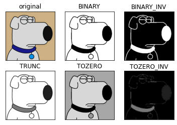
三、阈值与平滑处理 1. 图像阈值ret, dst = cv2.threshold(src, thresh, maxval, type)参数说明:src:输入图(只能输入单通道图像,一般为灰度图)dst:输出图thresh:阈值maxval:当像素值大于/小于阈值(根据type决定大于/小于),所赋予的值type:二值化的操作类型,包含以下5种:cv2.THRESH_BINARY:超过阈值部分取maxval,否则取0cv2.THRESH_BINARY_INV:THRESH_BINARY取反cv2.THRESH_TRUNC:大于阈值的像素值设为阈值,其他的不变cv2.THRESH_TOZERO:大于阈值的像素值不变,其他的设为0cv2.THRESH_TOZERO_INV:THRESH_TOZERO取反import cv2 # OpenCV 读取的格式是 BGR import matplotlib.pyplot as plt import numpy as np %matplotlib inline img = cv2.imread('ble.jpg') img_gray = cv2.imread('ble.jpg', cv2.IMREAD_GRAYSCALE) ret, thresh1 = cv2.threshold(img_gray, 127, 255, cv2.THRESH_BINARY) ret, thresh2 = cv2.threshold(img_gray, 127, 255, cv2.THRESH_BINARY_INV) ret, thresh3 = cv2.threshold(img_gray, 127, 255, cv2.THRESH_TRUNC) ret, thresh4 = cv2.threshold(img_gray, 127, 255, cv2.THRESH_TOZERO) ret, thresh5 = cv2.threshold(img_gray, 127, 255, cv2.THRESH_TOZERO_INV) titles = ['original', 'BINARY', 'BINARY_INV', 'TRUNC', 'TOZERO', 'TOZERO_INV'] images = [img, thresh1, thresh2, thresh3, thresh4, thresh5] for i in range(6): plt.subplot(2, 3, i + 1), plt.imshow(images[i], 'gray') plt.title(titles[i]) plt.xticks([]), plt.yticks([]) plt.show()2. 图像平滑img = cv2.imread('ysg.png') # cv2.imshow('img', img) # cv2.waitKey(0) # cv2.destroyAllWindows() plt.imshow(cv2.cvtColor(img, cv2.COLOR_BGR2RGB))<matplotlib.image.AxesImage at 0x2a857fb4d68># 均值滤波(平卷积操作) blur = cv2.blur(img, (5, 5)) # cv2.imshow('blur', blur) # cv2.waitKey(0) # cv2.destroyAllWindows() plt.imshow(cv2.cvtColor(blur, cv2.COLOR_BGR2RGB))<matplotlib.image.AxesImage at 0x2a8592e8c50># 方框滤波 # normalize=True 即选择归一化时和均值滤波一样 box_normalize_true = cv2.boxFilter(img, -1, (5, 5), normalize=True) # cv2.imshow('box_normalize_true', box_normalize_true) # cv2.waitKey(0) # cv2.destroyAllWindows() plt.imshow(cv2.cvtColor(box_normalize_true, cv2.COLOR_BGR2RGB))<matplotlib.image.AxesImage at 0x2a8592532b0># normalize=False 不做归一化,矩阵中的像素值相加,超过255取255 box_normalize_false = cv2.boxFilter(img, -1, (5, 5), normalize=False) # cv2.imshow('box_normalize_false', box_normalize_false) # cv2.waitKey(0) # cv2.destroyAllWindows() plt.imshow(cv2.cvtColor(box_normalize_false, cv2.COLOR_BGR2RGB))<matplotlib.image.AxesImage at 0x2a8579eed30># 高斯滤波 gaussian = cv2.GaussianBlur(img, (5, 5), 1) # cv2.imshow('gaussian', gaussian) # cv2.waitKey(0) # cv2.destroyAllWindows() plt.imshow(cv2.cvtColor(gaussian, cv2.COLOR_BGR2RGB))<matplotlib.image.AxesImage at 0x2a857a7b828># 中值滤波 median = cv2.medianBlur(img, 5) # cv2.imshow('median', median) # cv2.waitKey(0) # cv2.destroyAllWindows() plt.imshow(cv2.cvtColor(median, cv2.COLOR_BGR2RGB))<matplotlib.image.AxesImage at 0x2a8579d0588>
-
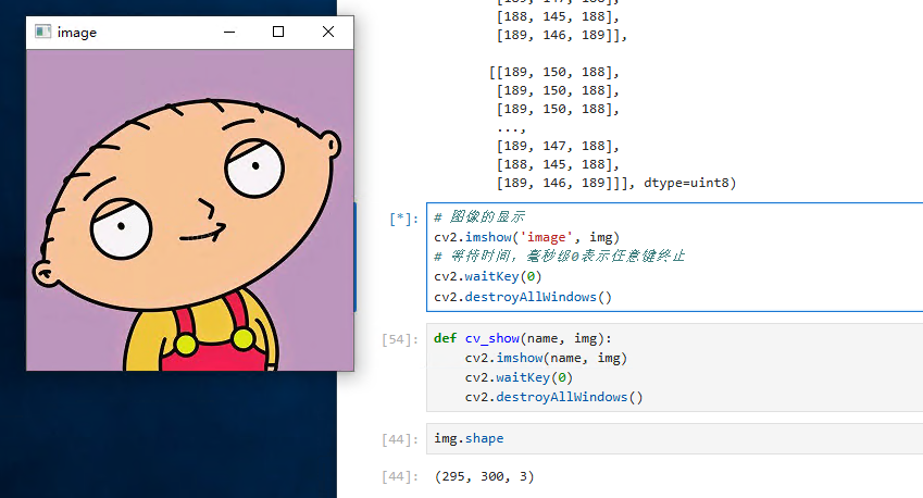
二、图像基本操作 1. 图像的读取与显示cv2.IMREAD_COLOR 彩色图像cv2.IMGREAD_GRAYSCALE 灰度图像import cv2 # OpenCV 读取的格式是 BGR import matplotlib.pyplot as plt import numpy as np %matplotlib inline img = cv2.imread('test.jpg') # 执行 img 回车可显示该图像的数据 array([[[189, 150, 188], [189, 150, 188], [188, 149, 187], ..., [189, 147, 188], [188, 146, 187], [189, 146, 189]], [[189, 150, 188], [188, 149, 187], [188, 149, 187], ..., [189, 147, 188], [188, 146, 187], [189, 146, 189]], [[188, 149, 187], [188, 149, 187], [188, 149, 187], ..., [189, 147, 188], [188, 146, 187], [189, 146, 189]], ..., [[189, 150, 188], [189, 150, 188], [189, 150, 188], ..., [189, 147, 188], [188, 146, 187], [189, 146, 189]], [[189, 150, 188], [189, 150, 188], [189, 150, 188], ..., [189, 147, 188], [188, 145, 188], [189, 146, 189]], [[189, 150, 188], [189, 150, 188], [189, 150, 188], ..., [189, 147, 188], [188, 145, 188], [189, 146, 189]]], dtype=uint8)# 图像的显示 cv2.imshow('image', img) # 等待时间,毫秒级0表示任意键终止 cv2.waitKey(0) cv2.destroyAllWindows()def cv_show(name, img): cv2.imshow(name, img) cv2.waitKey(0) cv2.destroyAllWindows()# 执行 img.shape 可输出该图像的 shape 数据 img.shape (295, 300, 3)# 读取灰度图 img = cv2.imread('test.jpg', cv2.IMREAD_GRAYSCALE) img array([[166, 166, 165, ..., 164, 163, 164], [166, 165, 165, ..., 164, 163, 164], [165, 165, 165, ..., 164, 163, 164], ..., [166, 166, 166, ..., 164, 163, 164], [166, 166, 166, ..., 164, 163, 164], [166, 166, 166, ..., 164, 163, 164]], dtype=uint8)# 图像的显示(灰度图) cv2.imshow('image', img) # 等待时间,毫秒级0表示任意键终止 cv2.waitKey(0) cv2.destroyAllWindows()# 保存 cv2.imwrite('test1.jpg', img)type(img) numpy.ndarray2. 读取视频cv2.VideoCapture 可以捕获摄像头,用数字来控制不同的设备,如:0,1如果是视频文件,可以直接指定路径vc = cv2.VideoCapture('jswyn.mp4') if vc.isOpened(): open, frame = vc.read() else: open = False while open: ret, frame = vc.read() if frame is None: break if ret == True: gray = cv2.cvtColor(frame, cv2.COLOR_BGR2GRAY) cv2.imshow('result', gray) if cv2.waitKey(10) & 0xFF == 27: break vc.release() cv2.destroyAllWindows()3. 截取部分图像数据(ROI区域)img = cv2.imread('test.jpg') jiaozi = img[0:50, 0: 150] cv_show('jiaozi', jiaozi)4. 颜色通道提取b,g,r = cv2.split(img) r array([[188, 188, 187, ..., 188, 187, 189], [188, 187, 187, ..., 188, 187, 189], [187, 187, 187, ..., 188, 187, 189], ..., [188, 188, 188, ..., 188, 187, 189], [188, 188, 188, ..., 188, 188, 189], [188, 188, 188, ..., 188, 188, 189]], dtype=uint8) r.shape (295, 300)# 合并 img = cv2.merge((b,g,r)) img.shape (295, 300, 3)# 只保留 R 通道 cur_img = img.copy() cur_img[:,:,0] = 0 cur_img[:,:,1] = 0 cv_show('R', cur_img)# 只保留 G 通道 cur_img = img.copy() cur_img[:,:,0] = 0 cur_img[:,:,2] = 0 cv_show('G', cur_img)# 只保留 B 通道 cur_img = img.copy() cur_img[:,:,1] = 0 cur_img[:,:,2] = 0 cv_show('B', cur_img)5. 边界填充top_size,bottom_size,left_size,right_size = (50, 50, 50, 50) replicate = cv2.copyMakeBorder(img, top_size, bottom_size, left_size, right_size, borderType=cv2.BORDER_REPLICATE) reflect = cv2.copyMakeBorder(img, top_size, bottom_size, left_size, right_size, borderType=cv2.BORDER_REFLECT) reflect101 = cv2.copyMakeBorder(img, top_size, bottom_size, left_size, right_size, borderType=cv2.BORDER_REFLECT_101) wrap = cv2.copyMakeBorder(img, top_size, bottom_size, left_size, right_size, borderType=cv2.BORDER_WRAP) constant = cv2.copyMakeBorder(img, top_size, bottom_size, left_size, right_size, borderType=cv2.BORDER_CONSTANT, value=0)import matplotlib.pyplot as plt plt.subplot(231), plt.imshow(img, 'gray'), plt.title('ORIGINAL') # plt.subplot(231), plt.imshow(replicate, 'gray'), plt.title('REPLICATE') # plt.subplot(231), plt.imshow(reflect, 'gray'), plt.title('REFLECT') # plt.subplot(231), plt.imshow(reflect101, 'gray'), plt.title('REFLECT_101') # plt.subplot(231), plt.imshow(wrap, 'gray'), plt.title('WRAP') # plt.subplot(231), plt.imshow(constant, 'gray'), plt.title('CONSTANT') plt.show()BORDER_REPLICATE:复制法,复制最边缘像素BORDER_REFLECT:反射法,对感兴趣的图像中的像素在两边进行复制,如:dcba|abcde|edcBORDER_REFLECT_101:反射法,以最边缘像素为轴,对称复制,如:dcb|abcd|cbaBORDER_WRAP:外包装法,如:bcde|abcde|abcdBORDER_CONSTANT:常量法,常量数值进行填充6. 数值计算img_jz = cv2.imread('test.jpg') img_jz[:5,:,0] array([[189, 189, 188, ..., 189, 188, 189], [189, 188, 188, ..., 189, 188, 189], [188, 188, 188, ..., 189, 188, 189], [188, 188, 188, ..., 189, 188, 189], [188, 188, 188, ..., 189, 188, 189]], dtype=uint8)img_jz1 = img_jz + 10 img_jz1[:5,:,0] array([[199, 199, 198, ..., 199, 198, 199], [199, 198, 198, ..., 199, 198, 199], [198, 198, 198, ..., 199, 198, 199], [198, 198, 198, ..., 199, 198, 199], [198, 198, 198, ..., 199, 198, 199]], dtype=uint8)# 相加时如果像素点的数值超过边界 255,则会将该值与256进行 % 取余操作 (img_jz + img_jz1)[:5,:,0] array([[132, 132, 130, ..., 132, 130, 132], [132, 130, 130, ..., 132, 130, 132], [130, 130, 130, ..., 132, 130, 132], [130, 130, 130, ..., 132, 130, 132], [130, 130, 130, ..., 132, 130, 132]], dtype=uint8)# 通过cv2的add方法进行操作时,如果像素点的数值超过边界 255,则取255,否则取它自身 cv2.add(img_jz,img_jz1)[:5,:,0] array([[255, 255, 255, ..., 255, 255, 255], [255, 255, 255, ..., 255, 255, 255], [255, 255, 255, ..., 255, 255, 255], [255, 255, 255, ..., 255, 255, 255], [255, 255, 255, ..., 255, 255, 255]], dtype=uint8)7. 图像融合# 当两张图的大小不一致时,无法进行融合,先用cv2.resize()方法调整 img_ble = cv2.imread('ble.jpg') img_jz + img_ble array([[[139, 68, 57], [140, 69, 58], [137, 68, 59], ..., [139, 70, 55], [138, 69, 53], [139, 69, 55]], [[140, 69, 58], [139, 68, 57], [137, 68, 59], ..., [139, 70, 55], [138, 69, 53], [139, 69, 55]], [[139, 68, 57], [139, 68, 57], [136, 67, 58], ..., [139, 70, 55], [138, 69, 53], [139, 69, 55]], ..., [[144, 68, 56], [137, 65, 57], [137, 70, 61], ..., [138, 68, 55], [137, 67, 54], [138, 68, 55]], [[143, 67, 55], [136, 64, 56], [135, 68, 59], ..., [138, 68, 55], [137, 66, 55], [139, 69, 56]], [[142, 66, 54], [141, 68, 60], [132, 65, 56], ..., [139, 69, 56], [138, 67, 56], [139, 69, 56]]], dtype=uint8)# 参数说明:img1,比例,img2,比例,亮度级 res = cv2.addWeighted(img_jz, 0.1, img_ble, 0.6, 0) plt.imshow(res)<matplotlib.image.AxesImage at 0x24ad14c8860># 将目标值设置为,通过x,y比例进行调整 res = cv2.resize(img, (0, 0), fx=3, fy=2.5) plt.imshow(res)<matplotlib.image.AxesImage at 0x24ad4d2f4e0>
-
一、环境配置 参考 b 站人工智能算法工程师 up 主1. 安装Anaconda下载地址:https://www.anaconda.com/download安装后使用 Python3.6 虚拟环境及 opencv-python 3.4.1.15 版本# 注:以管理员身份运行 Anaconda Prompt conda create -p C:\ProgramData\anaconda3\envs\py36 python=3.6 conda activate C:\ProgramData\anaconda3\envs\py36 pip install opencv-python==3.4.1.15 # 验证 opncv cd /d C:\ProgramData\anaconda3\envs\py36 python ipmort cv2 cv2.__version__安装拓展pip install opencv-contrib-python==3.4.1.152. Notebook安装并切换 Python3.6 内核# 继续在刚刚的 Anaconda Prompt 命令行窗口中执行以下代码 pip install ipykernel python -m ipykernel install --user --name py36 --display-name "Python 3.6 (py36)"打开 Jupyter Notebook,通过 http://localhost:8888/tree 可以访问到网页版 Notebook新建一个python测试文件,在顶部的 kernel 选项卡中可找到切换内核选项,切换至刚刚安装的 3.6 版本
-
Typecho Redis缓存插件 这个插件一直断断续续的在写着,功能不多(刚好够用,代码的 java 味儿略重,狗头)github地址:https://github.com/suaxi/TypechoRedisCache已实现功能:首次访问时缓存文章的 cid、标题、分类、创建/修改时间、作者、内容(Redis 数据类型为 Hash)已缓存文章数量统计清除全部缓存清除指定文章缓存(通过文章 cid)禁用插件时清除所有缓存后续计划:优化 Redis 配置选项2025-10-18 更新:添加 服务端连接配置 优化2025-10-20 更新:添加可选密码配置(生产环境建议将 Redis 外网权限隔离,仅在内网使用)
-
动画 1. requestAnimationFrame<!DOCTYPE html> <html lang="en"> <head> <meta charset="UTF-8"> <meta name="viewport" content="width=device-width, initial-scale=1.0"> <title>requestAnimationFrame</title> </head> <body> <script> // 1.创建 canvas 画布 const canvas = document.createElement('canvas') // 设置宽高 canvas.width = 500 canvas.height = 500 document.body.append(canvas) // 2.获取 context 对象(画笔) const context = canvas.getContext('2d') context.fillStyle = 'skyblue' // 画一个方形,使之随时间左右移动 // 调用 requestAnimationFrame 函数,使函数循环执行 let x = 0 function loop() { context.clearRect(0, 0, canvas.width, canvas.height) context.fillRect(x, 100, 100, 100, 100) x += 1 requestAnimationFrame(loop) } requestAnimationFrame(loop) </script> </body> </html>2. 环绕动画 - 行星运动<!DOCTYPE html> <html lang="en"> <head> <meta charset="UTF-8"> <meta name="viewport" content="width=device-width, initial-scale=1.0"> <title>环绕动画-行星运动</title> <style> canvas { background-color: #4d5053; /* color: #4d5053; */ } </style> </head> <body> <script> // 1.创建 canvas 画布 const canvas = document.createElement('canvas') // 设置宽高 canvas.width = 500 canvas.height = 500 document.body.append(canvas) // 2.获取 context 对象(画笔) const context = canvas.getContext('2d') // 地球旋转的角度 let earthAngle = 0 // 月球旋转的角度 let moonAngle = 0 function loop() { context.save() context.clearRect(0, 0, canvas.width, canvas.height) // 太阳 context.beginPath() context.arc(250, 250, 60, 0, 2 * Math.PI) context.fillStyle = '#f1ce07' context.shadowColor = '#f1ce07' context.shadowBlur = 10 context.fill() context.closePath() // 地球 // 1. 将canvas的原点移至太阳的中心 context.beginPath() context.translate(250, 250) context.rotate(earthAngle * Math.PI / 180) // 2. 将canvas的原点移至地球的中心(使日-地-月的中心在一条水平线上) context.translate(170, 0) context.arc(0, 0, 15, 0, 2 * Math.PI) context.fillStyle = 'blue' context.shadowBlur = 0 context.fill() earthAngle += 0.3 context.closePath() // 月亮 context.beginPath() context.rotate(moonAngle * Math.PI / 180) context.arc(35, 0, 6, 0, 2 * Math.PI) context.fillStyle = 'white' context.shadowBlur = 0 context.fill() moonAngle += 1.3 context.closePath() context.restore() requestAnimationFrame(loop) } requestAnimationFrame(loop) </script> </body> </html>