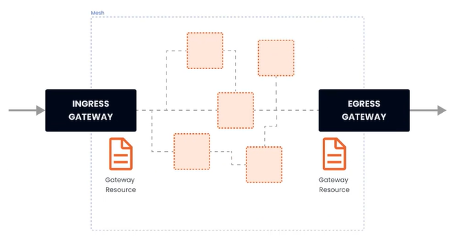
四、流量管理 - Gateway 在安装 istio 的时候，同时安装了入口和出口网关，这两个网关都运行了一个 Envoy 代理实例，它们在网格的边缘作为负载均衡器的角色。gateway 资源实例：apiVersion: networking.istio.io/v1alpha3 kind: Gateway metadata: name: gateway-demo namespace: default spec: selector: istio: ingressgateway servers: - port: number: 80 name: http protocol: HTTP hosts: - dev.example.com - test.example.com 上述示例做了哪些事：配置了一个代理，作为负载均衡器服务端口为80应用于 istio 入口网关代理hosts 字段作为过滤器，只有以 dev.example.com 和 test.example.com 为目的地的流量才允许通过为了控制和转发流量到集群内运行的实际实例，还需要配置 VirtualService，并与网关相连接。（1）简单路由实例部署 nginx，并通过 istio 网关进行访问--- apiVersion: apps/v1 kind: Deployment metadata: namespace: test name: nginx labels: app: nginx spec: replicas: 1 selector: matchLabels: app: nginx template: metadata: labels: app: nginx spec: restartPolicy: Always containers: - image: 'nginx:latest' imagePullPolicy: IfNotPresent name: nginx env: - name: TZ value: Asia/Shanghai ports: - containerPort: 80 protocol: TCP --- apiVersion: v1 kind: Service metadata: namespace: test name: nginx labels: app: nginx spec: ports: - port: 80 targetPort: 80 protocol: TCP selector: app: nginx# 网关 apiVersion: networking.istio.io/v1alpha3 kind: Gateway metadata: name: gateway-nginx namespace: test spec: selector: istio: ingressgateway servers: - port: number: 80 name: http protocol: HTTP hosts: - '*'在未绑定 VirtualService 之前，网关还不知道要将流量路由到哪apiVersion: networking.istio.io/v1alpha3 kind: VirtualService metadata: name: virtualService-nginx namespace: test spec: hosts: - '*' gateways: - gateway-nginx http: - route: - destination: host: nginx.test.svc.cluster.local port: 80部署完之后，通过 curl -v x.x.x.x 即可测试

三、安装 以 istioctl 为例# 下载 curl -L https://istio.io/downloadIstio | sh - cd istio-1.28.1 export PATH=$PWD/bin:$PATH安装目录包含：samples/ 目录下的示例应用bin/ 目录下的 istioctl 客户端可执行文件。# 安装 istioctl install --set profile=demo -y |\ | \ | \ | \ /|| \ / || \ / || \ / || \ / || \ / || \ /______||__________\ ____________________ \__ _____/ \_____/ √ Istio core installed √ Istiod installed √ Ingress gateways installed √ Egress gateways installed √ Installation complete istio 提供的几种内置配置，这些配置文件提供了对 Istio 控制平面和 Istio 数据平面 Sidecar 的定制内容:default：根据 IstioOperator API 的默认设置启动组件。 建议用于生产部署和 Multicluster Mesh 中的 Primary Cluster。您可以运行 istioctl profile dump 命令来查看默认设置。demo：这一配置具有适度的资源需求，旨在展示 Istio 的功能。 它适合运行 Bookinfo 应用程序和相关任务。 此配置文件启用了高级别的追踪和访问日志，因此不适合进行性能测试。minimal：与默认配置文件相同，但只安装了控制平面组件， 它允许您使用 Separate Profile 配置控制平面和数据平面组件(例如 Gateway)。remote：配置 Multicluster Mesh 的 Remote Cluster。empty：不部署任何东西。可以作为自定义配置的基本配置文件。preview：预览文件包含的功能都是实验性。这是为了探索 Istio 的新功能，不确保稳定性、安全性和性能（使用风险需自负）。 defaultdemominimalremoteemptypreview核心组件 istio-egressgateway √ istio-ingressgateway√√ √istiod√√√ √# 给命名空间添加标签，指示 Istio 在部署应用的时候，自动注入 Envoy Sidecar 代理 kubectl label namespace [default] istio-injection=enabled安装 Kubernetes Gateway API CRDKubernetes Gateway API CRD 在大多数 Kubernetes 集群上不会默认安装， 在使用 Gateway API 之前需要安装$ kubectl get crd gateways.gateway.networking.k8s.io &> /dev/null || \ { kubectl kustomize "github.com/kubernetes-sigs/gateway-api/config/crd?ref=v1.4.0" | kubectl app

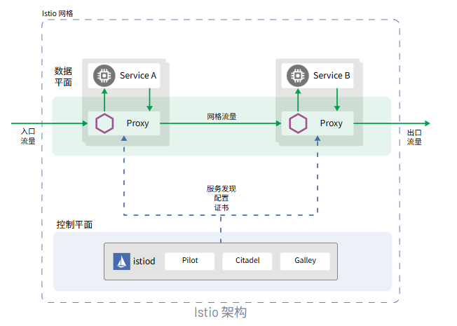
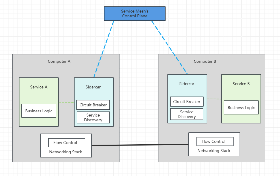
二、Istio 官网：https://istio.io/latest/zh/Istio 是一种开源服务网格，可透明地分层到现有的分布式应用程序上。 Istio 的强大功能提供了一种统一且更高效的方式来保护、连接和监控服务。 Istio 是实现负载均衡、服务到服务身份验证和监控的途径 - 几乎无需更改服务代码。包含以下功能：使用双向 TLS 加密、强大的基于身份的身份验证和鉴权在集群中保护服务到服务通信HTTP、gRPC、WebSocket 和 TCP 流量的自动负载均衡使用丰富的路由规则、重试、故障转移和故障注入对流量行为进行细粒度控制支持访问控制、限流和配额的可插入策略层和配置 API集群内所有流量（包括集群入口和出口）的自动指标、日志和链路追踪Istio 服务网格从逻辑上划分为数据平面和控制平面数据平面：由一组被部署为 Sidercar 的智能代理（Envoy）组成，负责协调和控制微服务之间的所有网络通信，同时也收集和报告所有网格流量的遥测数据控制平面：管理、配置代理，进行流量路由

一、服务网格 服务网格（Service Mesh）是一个专用的基础架构层，用于管理分布式应用程序中各个微服务之间的通信。它充当透明且分散的代理网络，并且部署在应用服务旁边，这些代理通常被称为 Sidercar，用于处理服务间的网络调用，限流，熔断，负载均衡等。当微服务（Service）集群扩大到一定规模后，就形成了网格状（Mesh），即 Service Mesh 形态

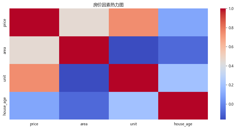
二、数据分析 - seaborn - 案例 1. 房地产市场洞察与数据评估（1）导入依赖（2）导入数据（3）数据概览（4）数据清洗（5）新数据特征构造（6）问题分析及可视化import numpy as np import matplotlib.pyplot as plt import pandas as pd import seaborn as sns import datetime from matplotlib import rcParams rcParams['font.family'] = 'Microsoft YaHei'df = pd.read_csv('static/2_pandas/data/house_sales.csv', encoding='utf-8') print("总记录数：", len(df)) print("字段数数：", len(df.columns)) print(df.head(10)) print() df.info() 总记录数： 106118 字段数数： 12 city address area floor name price province \ 0 合肥 龙岗-临泉东路和王岗大道交叉口东南角 90㎡ 中层（共18层） 圣地亚哥 128万 安徽 1 合肥 龙岗-临泉东路和王岗大道交叉口东南角 90㎡ 中层（共18层） 圣地亚哥 128万 安徽 2 合肥 生态公园-淮海大道与大众路交口 95㎡ 中层（共18层） 正荣·悦都荟 132万 安徽 3 合肥 生态公园-淮海大道与大众路交口 95㎡ 中层（共18层） 正荣·悦都荟 132万 安徽 4 合肥 撮镇-文一名门金隅裕溪路与东风大道交口 37㎡ 中层（共22层） 文一名门金隅 32万 安徽 5 合肥 撮镇-文一名门金隅裕溪路与东风大道交口 37㎡ 中层（共22层） 文一名门金隅 32万 安徽 6 合肥 龙岗-长江东路与和县里交口 50㎡ 高层（共30层） 柏庄金座 46万 安徽 7 合肥 龙岗-长江东路与和县里交口 50㎡ 高层（共30层） 柏庄金座 46万 安徽 8 合肥 新亚汽车站-张洼路与临泉路交汇处向北100米(原红星机械 120㎡ 中层（共27层） 天目未来 158万 安徽 9 合肥 新亚汽车站-张洼路与临泉路交汇处向北100米(原红星机械 120㎡ 中层（共27层） 天目未来 158万 安徽 rooms toward unit year \ 0 3室2厅 南北向 14222元/㎡ 2013年建 1 3室2厅 南北向 14222元/㎡ 2013年建 2 3室2厅 南向 13895元/㎡ 2019年建 3 3室2厅 南向 13895元/㎡ 2019年建 4 2室1厅 南北向 8649元/㎡ 2017年建 5 2室1厅 南北向 8649元/㎡ 2017年建 6 2室1厅 南向 9200元/㎡ 2019年建 7 2室1厅 南向 9200元/㎡ 2019年建 8 4室2厅 南向 13167元/㎡ 2012年建 9 4室2厅 南向 13167元/㎡ 2012年建 origin_url 0 https://hf.esf.fang.com/chushou/3_404230646.htm 1 https://hf.esf.fang.com/chushou/3_404230646.htm 2 https://hf.esf.fang.com/chushou/3_404304901.htm 3 https://hf.esf.fang.com/chushou/3_404304901.htm 4 https://hf.esf.fang.com/chushou/3_404372096.htm 5 https://hf.esf.fang.com/chushou/3_404372096.htm 6 https://hf.esf.fang.com/chushou/3_398859799.htm 7 https://hf.esf.fang.com/chushou/3_398859799.htm 8 https://hf.esf.fang.com/chushou/3_381138154.htm 9 https://hf.esf.fang.com/chushou/3_381138154.htm <class 'pandas.core.frame.DataFrame'> RangeIndex: 106118 entries, 0 to 106117 Data columns (total 12 columns): # Column Non-Null Count Dtype --- ------ -------------- ----- 0 city 106118 non-null object 1 address 104452 non-null object 2 area 105324 non-null object 3 floor 104024 non-null object 4 name 105564 non-null object 5 price 105564 non-null object 6 province 106118 non-null object 7 rooms 104036 non-null object 8 toward 105240 non-null object 9 unit 105564 non-null object 10 year 57736 non-null object 11 origin_url 105564 non-null object dtypes: object(12) memory usage: 9.7+ MB# 数据清洗 df.drop(columns=['origin_url'], inplace=True) # df.head() # 缺失值处理 df.isna().sum() # 可选操作 df.dropna(inplace=True) # 删除重复数据 df.drop_duplicates(inplace=True) print(len(df)) 28104# 面积数据类型转换 df['area'] = df['area'].str.replace('㎡', '').astype(float) # 售价数据类型转换 df['price'] = df['price'].str.replace('万', '').astype(float) # 朝向数据类型转换 df['toward'] = df['toward'].astype('category') # 单价格数据类型转换 df['unit'] = df['unit'].str.replace('元/㎡', '').astype(float) # 年份格数据类型转换 df['year'] = df['year'].str.replace('年建', '').astype(int)# 异常值处理 # 房屋面积 df = df[(df['area'] > 20) & (df['area'] < 600)] # 价格 IQR Q1 = df['price'].quantile(0.25) Q3 = df['price'].quantile(0.75) IQR = Q3 - Q1 low_price = Q1 - 1.5 * IQR high_price = Q3 + 1.5 * IQR df = df[(df['price'] > low_price) & (df['price'] < high_price)]# 新数据特征构造 # 地区 district df['district'] = df['address'].str.split('-').str[0] # 楼层类型 floor_type df['floor_type'] = df['floor'].str.split('（').str[0].astype('category') # 是否是直辖市 zxs def is_zxs(city): if (city in ['北京', '上海', '天津', '重庆']): return True else: return False df['zxs'] = df['city'].apply(lambda x: 1 if is_zxs(x) else 0) # 卧室数 bedroom_num df['bedroom_num'] = df['rooms'].str.split('室').str[0].astype(int) # 客厅数量 living_room_num # df['living_room_num'] = df['rooms'].str.split('室').str[1].str.split('厅').str[0].fillna(0).astype(int) df['living_room_num'] = df['rooms'].str.extract(r'(\d+)厅').fillna(0).astype(int) # 房龄 house_age df['house_age'] = datetime.datetime.now().year - df['year'] # 价格区间 price_interval df['price_interval'] = pd.cut(df['price'], bins=3, labels=['低', '中', '高'])""" 分析一：哪些变量最影响房价？面积、楼层、房间数哪个因素影响最大？ 分析主题：特征性相关 分析目标：各因素对房价的线性影响 分组字段：无 指标/方法：皮尔逊相关系数 """ # 选择数值型特征 # corr() 相关系数 corr = df[['price', 'area', 'unit', 'house_age']].corr() print("影响房价的因素：") print(corr['price'].sort_values(ascending=False)[1:]) # 相关性热力图 plt.figure(figsize=(10, 5)) sns.heatmap(corr, cmap='coolwarm') plt.title('房价因素热力图') plt.tight_layout()影响房价的因素： unit 0.742731 area 0.452523 house_age 0.091520 Name: price, dtype: float64""" 分析二：全国房价的总体分布，是否存在极端值 分析主题：描述性统计 分析字段：概览数值型字段的分布特征 分组字段：无 指标/方法：平均数/中位数/四分位数/标准差 """ print(df.describe()) # 房价分布直方图 plt.subplot() plt.hist(df['price'], bins=10) area price unit year zxs \ count 26135.000000 26135.000000 26135.000000 26135.000000 26135.000000 mean 103.755810 117.208370 11610.131012 2013.072240 0.008800 std 33.995994 60.967675 5824.245273 6.019342 0.093399 min 21.000000 9.000000 1000.000000 1976.000000 0.000000 25% 85.005000 72.000000 7587.000000 2011.000000 0.000000 50% 100.000000 103.000000 10312.000000 2015.000000 0.000000 75% 123.000000 150.000000 14184.000000 2017.000000 0.000000 max 470.000000 306.000000 85288.000000 2023.000000 1.000000 bedroom_num living_room_num house_age count 26135.000000 26135.000000 26135.000000 mean 2.714444 1.848556 11.927760 std 0.800768 0.407353 6.019342 min 0.000000 0.000000 2.000000 25% 2.000000 2.000000 8.000000 50% 3.000000 2.000000 10.000000 75% 3.000000 2.000000 14.000000 max 9.000000 12.000000 49.000000 (array([ 991., 4810., 6499., 4613., 3362., 2226., 1333., 1055., 691., 555.]), array([ 9. , 38.7, 68.4, 98.1, 127.8, 157.5, 187.2, 216.9, 246.6, 276.3, 306. ]), <BarContainer object of 10 artists>)sns.histplot(data=df, x='price', bins=10, kde=True)<Axes: xlabel='price', ylabel='Count'>""" 分析三：南北向是否比单一朝向贵？贵多少？ 分析主题：朝向溢价 分析目标：评估不同朝向的价格差异 分组字段：toward 指标/方法：方差分析/多重比较 """ print(df['toward'].value_counts()) toward 南北向 14884 南向 8796 东南向 974 东向 419 北向 258 西南向 254 西向 161 东西向 151 西北向 133 东北向 105 Name: count, dtype: int64print(df.groupby('toward', observed=False).agg({ 'price': ['mean', 'median'], 'unit': 'median', 'house_age': 'mean' })) price unit house_age mean median median mean toward 东北向 114.555333 100.0 12198.0 12.609524 东南向 115.542608 105.0 10864.0 10.951745 东向 110.158568 95.0 11421.0 12.761337 东西向 98.935099 82.0 9000.0 15.490066 北向 92.527907 75.5 11698.0 13.108527 南北向 119.472147 104.5 10000.0 12.073703 南向 114.555016 103.0 10759.0 11.551160 西北向 119.107594 105.0 12290.0 13.473684 西南向 139.711811 138.4 13333.0 13.452756 西向 102.662298 86.0 12528.0 13.385093plt.figure(figsize=(10, 5)) sns.boxplot(data=df, x='toward', y='price') plt.tight_layout()

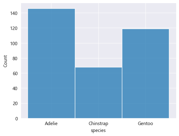
一、数据分析 - seaborn # 安装依赖 pip install seaborn一、统计图import pandas as pd import seaborn as sns import matplotlib.pyplot as plt from matplotlib import rcParams rcParams['font.family'] = 'Microsoft YaHei' # 设置图表大小 plt.figure(figsize=(10, 5)) # data penguins = pd.read_csv('static/2_pandas/data/penguins.csv') penguins.dropna(inplace=True) # penguins.head()1. 直方图sns.histplot(data=penguins, x='species') <Axes: xlabel='species', ylabel='Count'>2. 核密度估计图核密度估计图（KDE，Kernel Density Estimate Plot）用于显示数据分布，其通过平滑直方图的方法来估计数据的概率密度函数，使得分布图看起来更加连续、平滑。核密度估计是一种非参数方法，用于估计随机变量的概率密度函数。其基本思想是将每个数据点视为一个”核（高斯分布）“，然后将这些核的贡献相加以构成平滑的密度曲线。# 喙长度 - 核密度估计图 sns.kdeplot(data=penguins, x='bill_length_mm') <Axes: xlabel='bill_length_mm', ylabel='Density'>sns.histplot(data=penguins, x='bill_length_mm', kde=True) <Axes: xlabel='bill_length_mm', ylabel='Count'>3. 计数图计数图用于绘制分类变量的计数分布图，显示每个类别在数据集中出现的次数，可以快速了解类别的分布情况。# 不同岛屿的企鹅分布数量 sns.countplot(data=penguins, x='island') <Axes: xlabel='island', ylabel='count'>4. 散点图# x：体重，y：脚蹼长度 # hue参数可设置通过不同”分类“进行比对 sns.scatterplot(data=penguins, x='body_mass_g', y='flipper_length_mm', hue='sex') <Axes: xlabel='body_mass_g', ylabel='flipper_length_mm'>5. 蜂窝图# kind='hex' sns.jointplot(data=penguins, x='body_mass_g', y='flipper_length_mm', kind='hex') <seaborn.axisgrid.JointGrid at 0x239c7cddc40>6. 二维核密度估计图# 同时设置参数x和y sns.kdeplot(data=penguins, x='body_mass_g', y='flipper_length_mm') <Axes: xlabel='body_mass_g', ylabel='flipper_length_mm'># fill 填充 # cbar 颜色示意条 sns.kdeplot(data=penguins, x='body_mass_g', y='flipper_length_mm', fill=True, cbar=True) <Axes: xlabel='body_mass_g', ylabel='flipper_length_mm'>7. 条形图sns.barplot(data=penguins, x='species', y='bill_length_mm', estimator='mean', errorbar=None) <Axes: xlabel='species', ylabel='bill_length_mm'>8. 箱线图sns.boxplot(data=penguins, x='species', y='bill_length_mm') <Axes: xlabel='species', ylabel='bill_length_mm'>9. 小提琴图小提琴图（Violin Plot）是一种结合了箱线图和核密度估计图的可视化图表，用于展示数据的分布情况、集中趋势、散布情况以及异常值，不仅可以显示数据的基本统计量（中位数、四分位数等），还可以展示数据的概率密度。sns.violinplot(data=penguins, x='species', y='bill_length_mm') <Axes: xlabel='species', ylabel='bill_length_mm'>10. 成对关系图成对关系图是一种用于显示多个变量之间关系的可视化图表，其对角线上的图通常显示每个变量的分布，即单变量特性，其他位置的图用于展示所有变量的两两关系。sns.pairplot(penguins, hue='species') <seaborn.axisgrid.PairGrid at 0x239c979de20>

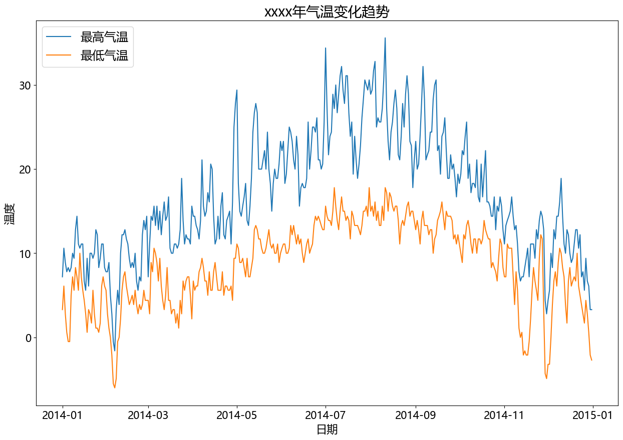
二、matplotlib - 统计图 - 案例 （1）温度、降水量分析import pandas as pd import matplotlib.pyplot as plt from matplotlib import rcParams rcParams['font.family'] = 'Microsoft YaHei' # data df = pd.read_csv('static/2_pandas/data/weather.csv') # print(df.head()) df['date'] = pd.to_datetime(df['date']) df = df[df['date'].dt.year == 2014] # 设置图表大小 plt.figure(figsize=(15, 10)) # 气温趋势变化图 plt.plot(df['date'], df['temp_max'], label='最高气温') plt.plot(df['date'], df['temp_min'], label='最低气温') plt.title('xxxx年气温变化趋势', fontsize=20) plt.legend(loc='upper left', fontsize='xx-large') plt.xlabel('日期', fontsize=16) plt.ylabel('温度', fontsize=16) plt.xticks(fontsize=15) plt.yticks(fontsize=15) plt.show()# 设置图表大小 plt.figure(figsize=(10, 5)) # 降水量直方图 data = df[df['date'].dt.year == 2014] plt.hist(data.precipitation, bins=5) plt.title('xxxx年降水量统计（直方图）', fontsize=16) plt.xlabel('降水量', fontsize=12) plt.ylabel('天数', fontsize=12) plt.show()

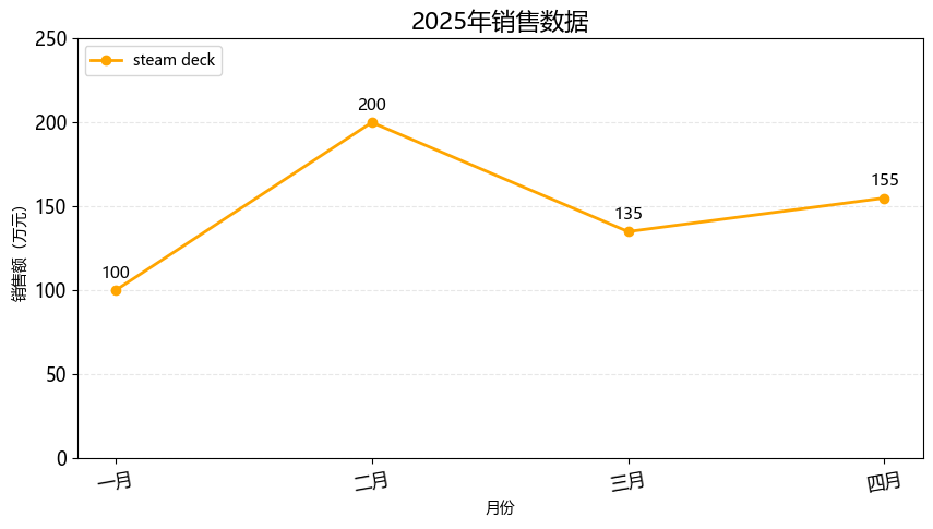
一、matplotlib - 统计图 # 安装依赖 pip install matplotlib1. 折线图import matplotlib.pyplot as plt from matplotlib import rcParams rcParams['font.family'] = 'Microsoft YaHei' # 设置图表大小 plt.figure(figsize=(10, 5)) month = ['一月', '二月', '三月', '四月'] sales = [100, 200, 135, 155] # 绘制折线图 plt.plot(month, sales, label='steam deck', color='orange', linewidth=2, marker='o') # 标题 plt.title('2025年销售数据', fontsize=16) # 坐标轴标签 plt.xlabel('月份') plt.ylabel('销售额（万元）') # 图例 plt.legend(loc='upper left') # 背景 plt.grid(axis='y', alpha=0.3, linestyle='--') # 设置刻度的样式（可选） plt.xticks(rotation=10, fontsize=12) plt.yticks(rotation=0, fontsize=12) # y轴范围 plt.ylim(0, 250) # 在每个坐标点上显示数值 for x, y in zip(month, sales): plt.text(x, y + 5, str(y), ha='center', va='bottom', fontsize=11) plt.show()2. 条形图import matplotlib.pyplot as plt from matplotlib import rcParams rcParams['font.family'] = 'Microsoft YaHei' # 设置图表大小 plt.figure(figsize=(10, 5)) subjects = ['语文', '数学', '英语', '思政'] scores = [93, 96, 60, 90] # bar 纵向柱状图 plt.bar(subjects, scores, label='学生：孙笑川', width=0.3) # 标题 plt.title('期末成绩', fontsize=16) # 坐标轴标签 plt.xlabel('科目') plt.ylabel('分数') # 图例 plt.legend(loc='upper left') # 背景 plt.grid(axis='y', alpha=0.3, linestyle='--') # 设置刻度的样式（可选） plt.xticks(rotation=0, fontsize=12) plt.yticks(rotation=0, fontsize=12) # y轴范围 plt.ylim(0, 100) # 在每个坐标点上显示数值 for x, y in zip(subjects, scores): plt.text(x, y + 5, str(y), ha='center', va='bottom', fontsize=11) # 自动优化排版 plt.tight_layout() plt.show()import matplotlib.pyplot as plt from matplotlib import rcParams rcParams['font.family'] = 'Microsoft YaHei' # 设置图表大小 plt.figure(figsize=(10, 5)) subjects = ['孙笑川', '药水哥', 'Giao哥', '刘波'] scores = [9.3, 9.6, 8.0, 9.0] # barh 横向柱状图 plt.barh(subjects, scores, label='成绩', color='orange') # 标题 plt.title('50米短跑成绩', fontsize=16) # 坐标轴标签 plt.xlabel('用时') plt.ylabel('学生') # 图例 plt.legend(loc='upper right') # 背景 plt.grid(axis='x', alpha=0.3, linestyle='--') # 设置刻度的样式（可选） plt.xticks(rotation=0, fontsize=12) plt.yticks(rotation=0, fontsize=12) # x轴范围 plt.xlim(0, 15) # 在每个坐标点上显示数值 for index, score in enumerate(scores): plt.text(score + 0.5, index, f'{score}', ha='left', va='bottom', fontsize=11) # 自动优化排版 plt.tight_layout() plt.show()3. 饼图import matplotlib.pyplot as plt from matplotlib import rcParams rcParams['font.family'] = 'Microsoft YaHei' # 设置图表大小 plt.figure(figsize=(10, 5)) things = ['看书', '电影', '游泳', '做饭', '其他'] times = [1.5, 2, 1, 2, 0.5] # 配色 colors = ['red', 'skyblue', 'green', 'orange', 'yellow'] # autopct 显示占比 # startangle 初始画图的角度 # colors 饼图配色 # wedgeprops 圆环半径 # pctdistance 百分比显示位置 plt.pie(times, labels=things, autopct='%.1f%%', startangle=90, colors=colors, wedgeprops={'width': 0.6}, pctdistance=0.6) # 标题 plt.title('每日活动时间分布', fontsize=16) plt.text(0, 0, '总计：100%', ha='center', va='bottom', fontsize=10) # 自动优化排版 plt.tight_layout() plt.show()import matplotlib.pyplot as plt from matplotlib import rcParams rcParams['font.family'] = 'Microsoft YaHei' # 设置图表大小 plt.figure(figsize=(10, 5)) things = ['看书', '电影', '游泳', '做饭', '其他'] times = [1.5, 2, 1, 2, 0.5] # 配色 colors = ['red', 'skyblue', 'green', 'orange', 'yellow'] # 爆炸式饼图，设置突出块 explode = (0, 0.2, 0.1, 0, 0.05) # autopct 显示占比 # startangle 初始画图的角度 # colors 饼图配色 # wedgeprops 圆环半径 # pctdistance 百分比显示位置 plt.pie(times, labels=things, autopct='%.1f%%', startangle=90, colors=colors, pctdistance=0.6, explode=explode, shadow=True) # 标题 plt.title('每日活动时间分布', fontsize=16) plt.text(0, 0, '总计：100%', ha='center', va='bottom', fontsize=10) # 自动优化排版 plt.tight_layout() plt.show()4. 散点图import matplotlib.pyplot as plt from matplotlib import rcParams rcParams['font.family'] = 'Microsoft YaHei' # 设置图表大小 plt.figure(figsize=(10, 5)) month = ['一月', '二月', '三月', '四月', '五月', '六月'] sales = [100, 200, 135, 155, 210, 235] # 绘制散点图 plt.scatter(month, sales) # 标题 plt.title('2025年上半年销售趋势', fontsize=16) # 自动优化排版 plt.tight_layout() plt.show()import matplotlib.pyplot as plt from matplotlib import rcParams import random rcParams['font.family'] = 'Microsoft YaHei' # 设置图表大小 plt.figure(figsize=(10, 5)) x = [] y = [] for i in range(500): temp = random.uniform(0, 10) x.append(temp) y.append(2 * temp + random.gauss(0, 2)) # 绘制散点图 plt.scatter(x, y, alpha=0.5, s=20, label='数据') # 标题 plt.title('x、y 变量趋势', fontsize=16) # 坐标轴标签 plt.xlabel('x变量') plt.ylabel('y变量') # 图例 plt.legend(loc='upper left') # 背景 plt.grid(True, alpha=0.3, linestyle='--') # 设置刻度的样式（可选） plt.xticks(rotation=0, fontsize=12) plt.yticks(rotation=0, fontsize=12) # y轴范围 # plt.ylim(0, 30) # 回归线 plt.plot([0, 10], [0, 20], color='red', linewidth=2) # 自动优化排版 plt.tight_layout() plt.show()5. 箱线图import matplotlib.pyplot as plt from matplotlib import rcParams rcParams['font.family'] = 'Microsoft YaHei' # 设置图表大小 plt.figure(figsize=(10, 5)) data = { "语文": [88, 82, 85, 89, 91, 80, 79, 83, 87, 89], "数学": [90, 91, 80, 67, 85, 88, 93, 96, 81, 89], "英语": [96, 88, 83, 45, 89, 73, 77, 80, 98, 66], } # 绘制箱线图 plt.boxplot(data.values(), tick_labels=data.keys()) # 标题 plt.title('各科成绩分布（箱线图）', fontsize=16) # 坐标轴标签 plt.xlabel('科目') plt.ylabel('分数') # 背景 plt.grid(True, alpha=0.3, linestyle='--') # 自动优化排版 plt.tight_layout() plt.show()6. 绘制多个图import matplotlib.pyplot as plt from matplotlib import rcParams rcParams['font.family'] = 'Microsoft YaHei' # 设置图表大小 plt.figure(figsize=(10, 5)) # data month = ['一月', '二月', '三月', '四月'] sales = [100, 200, 135, 155] # subplot 行 列 索引 p1 = plt.subplot(2, 2, 1) p1.plot(month, sales) p2 = plt.subplot(2, 2, 2) p2.bar(month, sales) p2 = plt.subplot(2, 2, 3) p2.scatter(month, sales) p2 = plt.subplot(2, 2, 4) p2.barh(month, sales)